

An imaginary rolling circle has taken us through intricate loops, exact repeating motion, rectangles, and ellipses. One obstacle remains between those equations and a piece of walnut: how do we store the curve?
Mathematics defines infinitely many positions along a path. A vector file needs a finite description.
Why not just connect the dots?
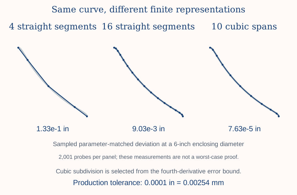
We could sample the equations and join the points with straight lines. Six chords make a poor approximation of a circle; sixty do better; thousands can look very smooth.
That approach is useful, but intricate curves may require many short segments. A design application has to process them, and a CAM system may translate them into numerous movements. The practical effect depends on the software, controller, and machining strategy.
We want a compact description that bends smoothly between its endpoints. Vector graphics already have a good tool for that.
Open the full-size diagram
Meet the Bézier curve
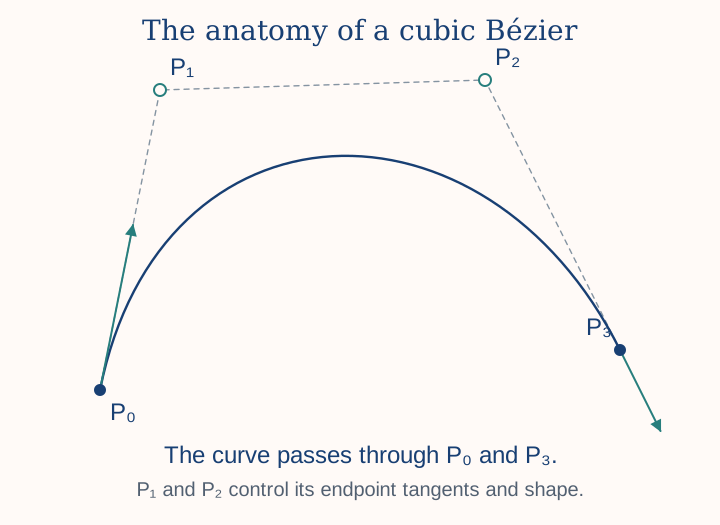
A cubic Bézier uses four control points. P₀ and P₃ are its endpoints; P₁ and P₂ control the departure and arrival directions and the shape between them. The two interior control points generally do not lie on the curve.
Open the full-size diagram
The local parameter u runs from zero to one. One cubic cannot reproduce every trochoid exactly, but a sequence of carefully chosen cubics can approximate it very closely.
We know more than where the curve is
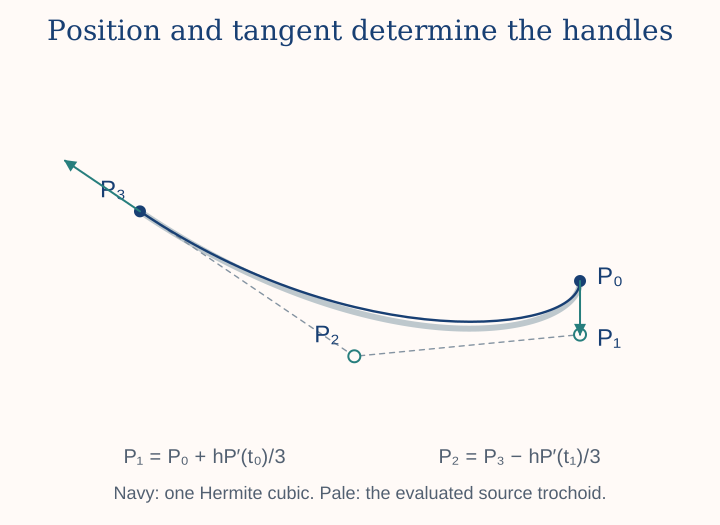
Our parametric equations provide both position P(t) and derivative P′(t). Away from a stationary point, the derivative tells us the tangent direction as well as the rate of change with the parameter.
For an interval from t0 to t1, write h = t1 − t0. Cubic Hermite interpolation gives Bézier controls directly:
The endpoints and endpoint derivatives match the source when expressed in the same parameter. At a smooth join, neighboring intervals therefore share their calculated endpoint and tangent direction. At a cusp, the zero derivative and deliberate sharp feature need special care rather than smoothing away.
Open the full-size diagram
How many segments are enough?
Too few segments allow the approximation to wander away from the source. Too many add complexity without useful benefit. An error bound gives us a principled choice.
Cubic Hermite error depends on the fourth derivative and the fourth power of the interval length. Halving an interval can reduce the corresponding bound by a factor of sixteen, provided the same derivative bound applies.
The circular generator chooses a subdivision from an analytic error bound, with evenly spaced parameter intervals within each lobe. It places rim-pen cusp locations at span boundaries. This is bound-selected subdivision, not a claim that every span is independently adapted to local curvature.
TRIV's elliptical fitter uses interval-dependent bounds and subdivision, with explicit boundaries at track-piece joins and rim-pen cusps. Different source geometry calls for different handling; the result is still a sequence of ordinary cubic Béziers.
One ten-thousandth of an inch
The precision vector output uses an interpolation target of:
This describes how closely the vector approximates its mathematical source at its intended output size. TRIV accounts for its own final scale factors when choosing the interpolation tolerance. Enlarging an exported vector later also enlarges its absolute approximation error; the original numerical tolerance is not a promise at every future size.
A sampled comparison is useful evidence that an implementation behaves as expected. It is not, by itself, proof of the greatest possible error between the samples. That is why analytic bounds matter.
Closing without an artificial seam
The underlying rolling construction closes before we serialize the vector. For circular curves, the final Bézier explicitly reuses the original starting point and derivative instead of relying on another trigonometric evaluation to produce bit-identical values.
TRIV first verifies the calculated closing position, then removes numerical roundoff by moving the final endpoint and its adjacent control point together. At a track-piece boundary, one-sided derivative magnitudes can differ even when tangent direction agrees; a closed path does not require pretending those magnitudes are identical.
An SVG close-path command records the closure, but it is not what makes the rolling mathematics periodic. We do not use it to conceal a missing portion of the intended curve.
From mathematics to SVG
Once the controls have been calculated, a design becomes something ordinary vector software can understand: a path made from cubic Bézier segments. SVG—Scalable Vector Graphics records those segments along with physical dimensions and other useful information.
The drawing is not tied to a pixel grid. Compatible editors and CAD/CAM applications can scale, combine, and work with it. Our native Vectric gadgets add the convenience of inserting the geometry directly into the design environment.
- EquationDescribe the rolling path.
- VectorApproximate it with controlled error.
- ToolpathChoose how a tool will follow it.
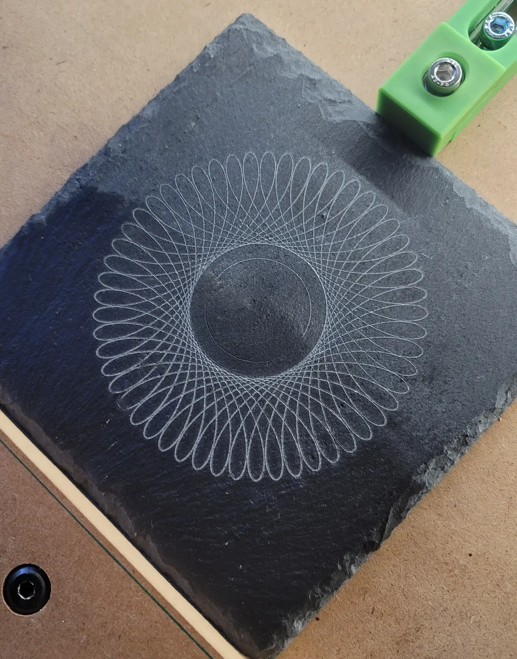
- EngravingLet the material have its say.
The adventure continues
Three measurements and a rolling circle have carried us through closure, unfamiliar tracks, and accurate interpolation into something we can make in the physical world.
The most interesting results don't always begin with knowing exactly what we want to create. Sometimes they begin with giving ourselves the tools to explore what might be possible.
That's the spirit behind Gadgetography. You're welcome to join us: try the PRIV Playground, browse the designs, or see what Millie has made of them.
A little further into the mathematics
- UC Berkeley's interpolation notes describe Hermite interpolation and its remainder.
- The W3C SVG paths specification defines cubic path segments and close-path behavior.